The Last 20 Years

I’ve been making fractal and algorithmic art for over 30 years now—since 1985. When I started, I did everything in a fairly random manner and didn’t keep many good notes. Then, when I began using Ultra Fractal in 1999, I started keeping pretty good records on the number of images and formulas I created. As I tallied the numbers for 2018, I realized that it’s been 20 years and that this would be a good time to look back and see what I’ve done.

Unfortunately (actually, fortunately), almost all of the images I made from 1985 through 1998 have been lost. But since 1/1/1999, I’ve kept every image that I thought was somehow interesting. Now, the vast majority of these aren’t suitable for publication (to my standards); this collection is more of a sketchbook—concepts, prototypes, false starts, dead ends, and first drafts. Yet, each was a completed image on its own, not just what happens when you open the program or just change one parameter. My sketchbook has 13,598 images! That’s about 680 per year, on average, or almost two per day, over 20 years. From this assemblage, I’ve culled 1,229 into my body of work—those that are (or will “soon” be) on my web site (along with 55 others that were completed before 1999).

If you’ve used Ultra Fractal, you know that a fractal image requires at least two formulas, one for the fractal shape and one for the coloring. Most of my images use formulas that I have written. When I began, there wasn’t much fractal software available, so I had to write my own programs, and I’ve never lost the love of that. As a result, I’ve written over 1,200 coloring formulas, almost 800 fractal formulas, and (only) 139 transformation formulas. Of these, 152 have been published in the Ultra Fractal Formula Database and amount to over 96,000 lines of code!

In these 20 years, in turns out that I’ve been actively involved in other aspects of fractal art, too. I’ve written, co-authored, or otherwise created 44 publications on math and/or art, from peer-reviewed research papers to my own books and art calendars. My images have appeared in 20 other publications, as illustrations and cover art. And I’ve reviewed dozens of other people’s papers and books.

It’s been quite a 20 years. And now, I need a nap. :-)

Digit Substitution Sequences

About three years ago, I played with a string substitution system based on the NATO phonetic alphabet. That system generated fractal sequences of words, but it did not easily lend itself to numbers.  So, recently I set out to find a similar system that worked with numbers.  The characteristics of the NATO system that I wanted this new thing to have were:

• It would be an iterative digit substitution scheme.  At each step, the digits in the previous iteration’s sequence would be substituted with others to create the next step’s sequence.
• The substitution rules would generally be the same for each digit, but might lead to different specific results, based on the value of the digit.
• The system would lead to a fractal sequence of digits.

As you might imagine, there are many ways to do this, depending on how the new numbers are generated from the old.  In order for this to work in a fashion similar to the NATO system, the new number needs to be a non-negative integer, just like the source numbers (the numbers 0, 1, 2, 3, 4, 5, 6, 7, 8, and 9).  For added interest, the new numbers should not all have the same number of digits, just like the words in the NATO phonetic alphabet do not all have the same number of letters.  One simple approach is to just square the original number, giving the substitutions shown in the table below.

Original	Substitution
0	0
1	1
2	4
3	9
4	16
5	25
6	36
7	49
8	64
9	81

Using this rule, nothing interesting happens beginning with 0 or 1.  The substitution is the same as the original numeral, so the sequence of numerals is 0, 0, 0, … or 1, 1, 1, …  Using 2 as a starting point yields some variation.  Here are the first several steps:

1. 4 (2 is replaced with 4)
2. 16 (4 is replaced with16)
3. 136 (the 1 is replaced with 1 and the 6 is replaced with 36)
4. 1936
5. 181936
6. 164181936
7. 13616164181936
8. 193613613616164181936
9. 1819361936193613613616164181936
10. 1641819361819361819361936193613613616164181936

There are some interesting patterns in this sequence.  From the second iteration on, the first digit is always 1, since 1 is replaced with 1 at each step.  Looking further, the first digits repeat every fourth iteration, in the pattern 16…, 13…, 19…, and 18…  Comparing the sixth and tenth iterations (for example), the entire sequence at the earlier step is repeated as the beginning of the later step (which is about five times as long).

Even though this series of sequences began with 2, 2 never shows up after that.  The only numerals that appear after the first few steps are:  1 (about one-third of the time), 3 (17%), 4 (5%), 6 (26%), 8 (8%), and 9 (11%).

On the back end, the same pattern of ending digits repeats and builds.  Aligning the 10 steps on the right shows this more clearly.  From the fifth step on, the entire previous sequence forms the end of the next sequence.

16

136

1936

181936

164181936

13616164181936

193613613616164181936

1819361936193613613616164181936

1641819361819361819361936193613613616164181936

136161641819361641819361641819361819361819361936193613613616164181936

This “back-end” sequence, except for the initial 1, can be constructed by using the same substitution scheme and beginning with 6 instead of 2 (6 becomes 36, which becomes 936, then 81936, etc.).  That 2 and 6 wind up with essentially the same patterns suggests what happens with other starting numerals.  Looking at the squares in the table above, 3 goes to 9, so 3 and 9 will lead to the same patterns.  The first numeral of 81 (9 × 9) is 8, so 9 and 8 will end up the same way.  And the first numeral of 64 (8 × 8) is 6, so 3, 6, 8, and 9 will all have the same destiny.  They will lead to sequences that begin with the same four sets of numerals, each repeating every fourth iteration:

•    36161641819361641819361641819361819361819361936193
•    64181936181936181936193619361361361616418193618193
•    81936193619361361361616418193619361361361616418193
•    93613613616164181936136161641819361361616418193616

Likewise, 2 × 2 is 4, so 2 and 4 will share the same path.  The first numerals of 25 (5 × 5) and 49 (7 × 7) are 2 and 4, so the starting points of 2, 4, 5, and 7 will all lead to the same results.  These patterns are the same as those for 3, 6, 8, and 9, except that these begin with 1.  The leading 1 has no impact on the rest of the sequences, but is simply carried on from one step to the next.

Other functions, aside from squaring, can be used and give different results.  For example, each numeral can be replaced with the cube of its number:

Original	Substitution
0	0
1	1
2	8
3	27
4	64
5	125
6	216
7	343
8	512
9	729

Here, as with squaring, beginning with 0 or 1 just leads to the same number again.  Since 2³ = 8, beginning with 2 or 8 results in the same pattern:
•    2
•    8
•    512
•    12518
•    181251512
•    151218125112518, etc.

The last digits build a pattern that repeats every second iteration, ending with 518 or 512.  Continuing a few more steps, the patterns grow to:
•    …51218125111812515121125181512181251151218125112518 and
•    …18125151211251815121812511125181512181251181251512

Inserting spaces between digits or groups of digits, you can see how, working from right to left,  concatenating the cubes of the digits in one sequence gives exactly the digits in the other, and vice versa.  In a sense each sequence creates the other.

•    …51218125111812515121125181512181 2 5 1 1 5 1 2 1 8 1 2 5 1 1 2 5 1 8
•    …18125151211251815121 8 125 1 1 125 1 8 1 512 1 8 125 1 1 8 125 1 512

•    …51218125111812515121 125 1 8 1 512 1 8 125 1 1 512 1 8 125 1 125 1 8
•    …18125151211251815121812511125181 5 1 2 1 8 1 2 5 1 1 8 1 2 5 1 5 1 2

The same thing happens with starting points of 3 and 7, but leading to two different sequences:

•    …83432166483435121812168121621664125188343216648343
•    …21681216216641812515125122764278121621664512276427

•    …83432166483435121812168121621664 1 2 5 1 8 8 3 4 3 2 1 6 6 4 8 3 4 3
•    …2168121621664 1 8 125 1 512 512 27 64 27 8 1 216 216 64 512 27 64 27

•    …8343216648343512 1 8 1 216 8 1 216 216 64 125 1 8 8 343 216 64 8 343
•    …21681216216641812515125122764278 1 2 1 6 2 1 6 6 4 5 1 2 2 7 6 4 2 7

The other four numbers, 4, 5, 6, and 9, give rise to their own sequences.  In these cases, each sequence generates itself.  Working right to left, replace each digit with its cube and you’ll recover the same sequence.  Alternatively, each group of digits that forms a perfect cube can be replaced by its cube root to get back to the same sequence.  For example, in 4’s sequence, starting from the right and replacing the last two digits (64) with 4 and each of the previous 216 with 6, gives 664, the last three digits of the sequence.

•    4:  …11251815121812161251815121812165121812168121621664
•    5:  …18125151211512181251125181181251512112518151218125
•    6:  …81251512115121812511251811812515121125181512181216
•    9:  …22764271812515128343216648343125182764275123438729

To generate images from all of these numbers, I used the same basic process described in the NATO post—drawing a series of line segments at different angles.  Take two sequences (not necessarily different).  March through the sequences one digit at a time.  The digit from the first sequence represents the angle to turn before drawing the segment and the digit from the second is the length of the segment.  In the image at the top of this post, I used the squaring sequence starting with 5 to determine the lengths and the cubing sequence starting with 5 to determine the angles.  The cube digits were multiplied by 90° to make sure that all the angles were right angles.  For something completely different, this image used adding for both sequences.  Starting with 9, add 17 to each digit for the length.  For the angles, start with 7 and replace each digit with 19 times its value.  Then, multiply those digits by approximately 179.632149°.

Prime Permutations

A few years ago, I played with fractions whose denominators are full reptend primes.  The fractions have decimal expansions that repeat, as do most fractions.  However, the repeating block for one fraction with a given denominator of this type is permutation of that for another fraction with the same denominator.  For example, consider the denominator 7.  The decimal expansions of its proper fractions are:

1. 1/7 = 0.142857142857142857142857142857…
2. 2/7 = 0.285714285714285714285714285714…
3. 3/7 = 0.428571428571428571428571428571…
4. 4/7 = 0.571428571428571428571428571428…
5. 5/7 = 0.714285714285714285714285714285…
6. 6/7 = 0.857142857142857142857142857142…

In each case, the repeating block is in bold.  Notice that the block for 1/7, 142857, is the same as it is for 2/7 (285714), except permuted by two spots.  That is, if you take the “14” from the 1/7 block off of the front end and put it on the back end, then you have the block for 2/7.  Likewise, the blocks for 3/7 and 4/7 are permutations of each other by three places—between the two fractions, the first half and second half of the blocks are swapped.  There are six different cyclic permutations of the block 142857, one for each fraction.

The same thing happens with other fractions whose denominators are full reptend primes.  For example, 19 is a full reptend prime.  When used as a denominator, its fractions repeat with a block of 18 digits.  Here are some of them:

• 1/19 = 0.05263157894736842105263157894737…
• 4/19 = 0.21052631578947368421052631578947…
• 9/19 = 0.47368421052631578947368421052632…

Compared with the block for 1/19 (052631578947368421), that for 4/19 is shifted three places to the right, and that for 9/19 is shifted nine places, swapping the first and second halves of the 1/19 block.

The comparisons need not be only with the first fraction’s block; any block can be compared with any other block (for the same denominator) to find out how many places it has been shifted, relative to the reference block.  Let’s return to 7.  In the table below, each row is for one of the six proper fractions with a denominator of 7.  Each column is for the repeating block of one of the six fractions.  The cells, then, give the place in the decimal expansion (row) where the particular repeating block (column) shows up.  For example, the value in the cell for row 2/7 and column 1/7 is 5 (yellow highlight), meaning that 1/7’s repeating block (142857) appears beginning at the fifth place in 2/7’s decimal expansion.  Likewise, the 3 in the cell intersecting the 5/7 row and the 3/7 column (orange highlight) means that 3/7’s repeating block (428571) begins at the third place in 5/7’s decimal expansion.

Reference fraction	1/7 142857	2/7 285714	3/7 428571	4/7 471428	5/7 714285	6/7 857142
1/7 = 0.142857…	1	3	2	5	6	4
2/7 = 0.285714…	5	1	6	3	4	2
3/7 = 0.428571…	6	2	1	4	5	3
4/7 = 0.571428…	3	5	4	1	2	6
5/7 = 0.714285…	2	4	3	6	1	5
6/7 = 0.857142…	4	6	5	2	3	1

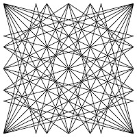
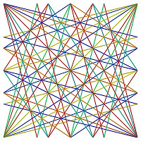
You may notice some patterns in the table.  The diagonal from the top left to the bottom right is all 1s.  This is because the reference fraction and the comparison block’s fraction are the same, so the comparison block always begins at the first place of its decimal expansion.  Also, the other diagonal, from the bottom left to the upper right, is all 4s.  In fact, all of the values in the table are arranged in diagonal bands, as this figure shows.  Each colored line shows a band for the same values, with each value being represented by a different color.  Extending the lines and removing the numbers and grid reveals the symmetry in the pattern.

 

Larger full reptend prime denominators have similar, but more detailed, patterns.  19 has 18 different proper fractions, as opposed to six for a denominator of 7.  Here is 19’s pattern, in black and white, to accentuate the structure, and in color to indicate the values.

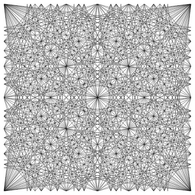
The relatively sparse areas in the center and at the corners give a hint as to what happens with larger denominators.  Here are the patterns for denominators of 61 and 193 (193’s is off-center to highlight the fractal detail).

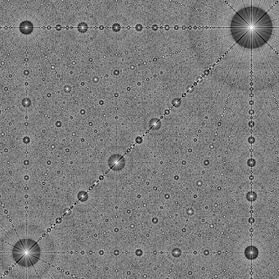
Finally, here is an image for a denominator of 1019, which is about the limit of my current system.

Round and Transform

When you round numbers, interesting things can happen.  For example, consider the fraction 6/11, 0.54545454…  When rounded to the nearest whole number, it rounds up to 1.  But when rounded to the nearest tenth, it rounds down to 0.5.  Nearest hundredth?  Up.  Nearest thousandth?  Down.  And so on.  Of course, numbers can be rounded in other ways.  Say, for example, 1/3, 0.33333…  It rounds down to the nearest whole number (0), up to the nearest half (0.5), down to the nearest quarter (0.25), up to the nearest eighth (0.375), etc.

The program Ultra Fractal, which I use for almost all of my fractal work, uses complex numbers and has a rounding function.  It rounds each part of the complex number (real and imaginary) to the nearest integer (positive, negative, or zero).  This can be used to round to any other number (say, nearest 2, nearest 0.5, or nearest π) by:

1. Decide on a rounding base.  For example, 1 for the nearest integer, 0.5 for the nearest half, or 3.14159... for the nearest π.
2. Multiply the number to be rounded by the rounding base.
3. Find the nearest complex integer for the scaled number found in step 2.
4. Divide the integer in step 3 by the rounding base.

To keep things interesting, I multiply the rounding base by a number each time.  For example, if I started with 1 and multiplied the base by 10 each iteration, then that would have the effect of rounding the number to the nearest 1, then to the nearest 10, then to the nearest 100, etc.  Also, I transform the rounded number in some fashion (say, rotate it and translate it) so that there’s something new to round in the next iteration.

Given all this goodness, there are lots of ways to create an image.  If the rounded number is different from the unrounded number, then there’s a rounding error at each iteration.  These can be accumulated and the image drawn according to some aspect of that total.  Larger rounding bases will generally have larger rounding errors (rounding 47 to the nearest 100 will have an error of 5, but rounding to the nearest 100 will have an error of -47), so the errors can be scaled by the rounding base before adding up.  You could just keep track of the direction of the rounding, say by adding 1 to a total if the number were rounded up and subtracting 1 if the number were rounded down.  Or, just color by the final rounded and transformed number, irrespective of what happened along the way.

The image at the top of the page begins with a rounding base of 0.0000152587890625 (2^-16) and doubles the base every iteration.  After rounding, the complex number is rotated by 31 degrees (not 30 or 32—31 is just right).

In the image above, the same rounding parameters are used, but this image is colored according to the relative rounding error (the image at the top uses the adding/subtracting 1 method).  And for this image, the complex number was rotated by 1 radian (about 57.3 degrees) each iteration.

This final example (above) uses the scaled increments and transforms the rounded number using the Mandelbrot set formula (z = z² + c).  This gives rise to the appearance of low-iteration Mandelbrot set fractal structures.

Fun with Modular Multiplicative Inverses

A regular multiplicative inverse (or just “inverse”) is the reciprocal of a number—the inverse of 2 is 1/2 and the inverse of 1/2 is 2.  The key property is that a number times its inverse equals 1.

Modular multiplicative inverses involve modular arithmetic, which involves the remainders of (typically whole) numbers when divided by a given base.  For example, 15 divided by 7 leaves a remainder of 1, so 15 = 1 modulo 7.  The phrase “modulo 7” means the remainder when divided by 7, and is often abbreviated “mod 7.”  Likewise, 22 = 6 mod 8 (remainder of 6 when 22 is divided by 8) and 143 = 3 mod 10 (remainder of 3 when 143 is divided by 10).

So modular multiplicative inverses combine the ideas of two numbers multiplying to 1 with the notion of the remainder, or mod.  The modular multiplicative inverse of a number is (the smallest) number such that the product of the two is 1, modulo some base.  For example, 3 x 5 = 15 and 15 = 1 mod 7.  So 3 and 5 are modular multiplicative inverses, for the base of 7.  For the base of 7, here are the modular multiplicative inverses:

Number	Inverse	Notes
0	none	Anything × 0 is 0, so the product will never have a remainder of 1.
1	1	1 × 1 = 1, for any base.
2	4	2 × 4 = 8, or 1 × 7 with a remainder of 1.
3	5	3 × 5 = 15, or 2 × 7 with a remainder of 1.
4	2	4 and 2 are inverses for base 7.
5	3	5 and 3 are inverses for base 7.
6	6	6 × 6 = 36, or 5 × 7 with a remainder of 1.
7	none	Anything × 7 will be a multiple of 7 and will have a remainder of 0.

The inverses depend on the base and some numbers will not have an inverse.  For example, with base 8:

Number	Inverse	Notes
0	none	Anything × 0 is 0, so the product will never have a remainder of 1.
1	1	1 × 1 = 1, for any base.
2	none	Anything × 2 will be even and will never have a remainder of 1.
3	3	3 × 3 = 9, or 1 × 8 with a remainder of 1.
4	none	Same as for 2.
5	5	5 × 5 = 25, or 3 × 8 with a remainder of 1.
6	none	Same as for 2.
7	7	7 × 7 = 48, or 6 × 8 with a remainder of 1.
8	none	Anything × 8 will be a multiple of 8 and will have a remainder of 0.

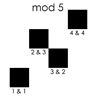
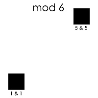
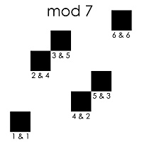
So what has this to do with the image?  Here are graphical representations of the modular multiplicative inverses for bases from 2 to 8.  In each image, the number and its inverse are plotted as squares in the (x, y) plane, where x is the number and y is its inverse.

  

The next image combines the previous seven by using the differences in colors of the corresponding pixels.  Black minus black is black, white minus white is black, and black minus white or white minus black is white.

Now, that image is combined with the one for mod 7, yielding this:

   

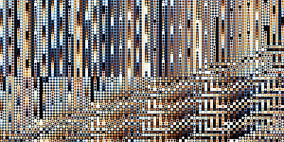
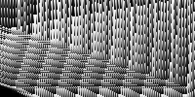
Finally, the one at the top of the page is a similar one, only using modulo bases 11 and 13.

Ratios of Subsequent Terms in Generalized Fibonacci Sequences

The Fibonacci sequence begins 0, 1, 1, 2, 3, 5, 8, etc.  Each subsequent term is the sum of the previous two.  As the terms get larger and larger, the ratio of two subsequent terms approaches a limit, the golden ratio or Φ, (1 + sqrt(5))/2, or about 1.6180339.  To see this, assume that each term is r times the previous term:  F_n+1 = r F_n, and F_n = r F_n-1.  Then, the Fibonacci recurrence equation

F_n+1 = F_n + F_n-1

becomes

r² F_n-1 = r F_n-1 + F_n-1, or
r² = r + 1.

The last equation is easily solved by the quadratic formula to give r = Φ.

This process can be extended to variations on the Fibonacci sequence by letting the new term be a weighted sum of the previous two terms:

F_n+1 = a F_n + b F_n-1

for some numbers a and b.  Then, by the same analysis, the ratio of subsequent terms will approach a limit r, r = (a + sqrt(a² + 4b))/2.  Here are some values of the ratio r for various a's and b's:

a	b	r
1	1	1.618
2	1	2.414
3	1	3.303
1	2	2
2	2	2.732
3	2	3.562
1	3	3
2	3	2.303
3	3	3.791

This table can be extended indefinitely.  Then, sort it by increasing values of r (when there is a tie, sort by increasing values of sqrt(a² + b²)).  This generates two sequences, A, the sequence of the a values, and B, the sequence of the b values.  The A sequence begins:

1, 1, 1, 2, 1, 2, 1, 2, 1, 1, 2, 3, 1, 2, 1, 3, 2, 1, 3, 2, 1, 3, 2, 1, 1, 2, 3, 4, 1, 2, 3, 1, 4, 2, 1, 3, 2, 4, 1, 3, 2, 1, 4, 3, 2, 1, 4, 3, 2, 1, 1, 2, 3, 4, 5, 1, 2, 3, 4, 1, 2, 5, 3, 1, 4, 2, 1, 3, 5, 2, 4, 1, 3, 2, 5, 1, 4, 3, 2, 1, 5, 4, 3, 2, 1, 5, 4, 3, 2, 1, 1, 2, 3, 4, 5, 6, 1, 2, 3, 4, …

and the B sequence begins:

1, 2, 3, 1, 4, 2, 5, 3, 6, 7, 4, 1, 8, 5, 9, 2, 6, 10, 3, 7, 11, 4, 8, 12, 13, 9, 5, 1, 14, 10, 6, 15, 2, 11, 16, 7, 12, 3, 17, 8, 13, 18, 4, 9, 14, 19, 5, 10, 15, 20, 21, 16, 11, 6, 1, 22, 17, 12, 7, 23, 18, 2, 13, 24, 8, 19, 25, 14, 3, 20, 9, 26, 15, 21, 4, 27, 10, 16, 22, 28, 5, 11, 17, 23, 29, 6, 12, 18, 24, 30, 31, 25, 19, 13, 7, 1, 32, 26, 20, 14, …

These sequences count each other--the terms in B count up how many times each number in A has shown up.  The first three terms of A are 1 and the first three terms of B count up the number of 1s in A.  Then, the fourth term of B is 1, indicating that the 2 that is the fourth term in A is the first time that a 2 shows up in A.  The fifth term of A is 1, which is the fourth 1 in A, and the fifth term of B is 4, to reflect that.  Likewise, the terms in A count up how many times each number is B has occurred.

All this relates to the image at the top of the page by considering the terms in A and B to be coordinates in the (x, y) plane and drawing segments from one point to the next.  The line begins in one corner, at point (1,1), then continues to (1,2), (1,3), (2,1), etc.  The image at the top has been rotated and flipped for aesthetic considerations; here is a blowup of the beginning of the curve oriented normally so you can follow it from point to point.

This post has been concerned with the principal solution of the quadratic equation, r = (a + sqrt(a² + 4b))/2.  But there is a second solution, r = (a - sqrt(a² + 4b))/2.  Here is the image corresponding to those values of r.

Space-Filled Popcorn

Pickover’s Popcorn algorithm is an iterative formula that doesn’t generate fractals in the typical way.  Because it typically uses trigonometric functions of real variables, instead of polynomials, there isn’t the standard inside/outside dichotomy of points.  Typically, none of the orbits diverge to infinity; they are either periodic or wander around a relatively small part of the plane.  Consequently, the Popcorn algorithm can be looked at as a warping of the complex plane.  This characteristic pairs nicely with the geometry of space-filling curves (like the Hilbert curve); they can be rendered to stay within a set region of the plane.

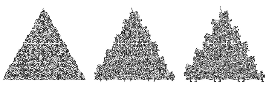
Here is the development of the image at the top of the screen, using this idea.  The first panel shows just a few iterations and the underlying Hilbert curve is clearly visible.  Then, with more and more iterations, the Popcorn swirls take over, obscuring any trace of the Hilbert curve.

Another approach uses a variation on the Hilbert curve.  The curve is based on triangles instead of squares, and starts like this.

Here’s the development of the curve, when combined with the Popcorn fractal:

And here’s the final image.

Metamorphosis

I have always been fascinated with Escher’s work, in particular his "Metamorphosis" woodcuts.  I’ve wanted to do something along those lines for years and finally came up with an approach.

I wrote my Scribble formula for Ultra Fractal in 2009, with something like this in mind, but I never made good use of it until now.  As you can read from the tutorial, Scribble essentially animates a rose curve along a path.  In these cases, the path was a horizontal line.  In the top image, the transition begins with a three-petal rose on the left, which morphs into a four-petal rose and then into a circle in the center.  From there, back to a three-petal rose and ending up with a four-petal rose curve.  The second image uses just four-petal roses of varying size (except for a circle in the center), and the final image uses only three-petal roses (plus a central circle).  In all, the phase angles associated with the sine and cosine functions are varied smoothly to impart a sense of rotation.

Julia Descending a Staircase

In my travels, I’ve become intrigued by the cubist style of painting and have wanted to make cubist fractals, whatever they are.  This is my first attempt. (In it, “Julia” refers to the Julia set fractal, not a particular woman.)  It was inspired by Duchamp's famous painting,"Nude Descending a Staircase." I created it using the embossing technqiue to get the minimal sense of the Julia sets, like Duchamp’s painting resembles sketches of the woman.  The Julia parameter changes slightly with each step, so the shapes vary down the staircase.  Also, I changed the lighting angle each step, to add more variation and to help distinguish the eight different Julia fractals.  None of them are entirely visible in the stack, like Duchamp's figures all kind of running over each other.  But I went from a more gray palette at the back (left) to black/white at the front (right) to help separate them and to give a sense of motion.

Random Walks with Pi

Much work has been done to create images from the digits of π (3.1415926…); in honor of Pi Day, here are a few of mine.

 

I generated a random walk using the first 10,000 digits of π (after the decimal point).  To do this, I let 0 be represented by a segment drawn to the right, 1 be a segment drawn 36 degrees counter-clockise from the horizontal; 2, 72 degrees and so on, up through 9, which is 324 degrees counter-clockwise (or 36 degrees clockwise).  It’s called a random walk because the path resembles what a person might do if walking around randomly.  The path begins in the red and ends in the blue.  Here is a magnification of the beginning, showing the first 1, at the lower center.

There’s no inherent reason to only use one digit at a time.  In the next walk, I took 20,000 digits in pairs, the first three being 14, 15, and 92.  Now, there are 100 different segment angles, each differing by 3.6 degrees from the next.

And finally, here is a walk using 50,000 digits, taken in groups of five (14159, 26535, etc.), for 100,000 possible angles.  Still looks random to me.

Concatenations, Part 2

In my last post, I talked about finding a string of 2,402 zeroes in the middle of the addition of the concatenation of 1, 2, 3, …, 960, 961, 962, plus the concatenation of 962, 961, 960, … , 3, 2, 1.  That is,

123456789 … 960961962 +
962961960 … 987654321 =
108641875 … [2402 zeroes] … 948616283.

With the wonderful help of Hans Havermann, I now understand how the string of zeroes came to appear there and seemingly nowhere else.

Let’s call x the maximum value in the concatenation (x = 962 here), A the ascending concatenation (A = 1123456789 … 960961962), and D the descending concatenation (D = 962961960 … 987654321).  When aligning A and D at the one’s place to add them (as we usually do), then the digits “960” from A pair up with “987” from D, as well as “961” with “654” and “962” with “321” at the very end on the right.  Working back to the left (down in A and up in D), the “900” from A lines up with “999” in D (from the number 99 and the first digit of 98).  From there (working left), both A and D have series of three-digit numbers, A going from 899 down to 100 and D going up from 100 to 899.  They all add up to a series of 10s, or a digit of 0 with a carry of 1.  Let’s look at a section:

A:       … ¹8 ¹9 ¹7 ¹8 ¹9 ¹8 ¹8 ¹9 ¹9 …
D:       …  1  0  2  1  0  1  1  0  0 …
sum:   …  0  0  0  0  0  0  0  0  0 …

(The superscript 1 indicates a carry from the previous column.)

From 100 to 899 is 800 numbers, each with three digits, for a total of 2,400 digits.  Then, when A goes from 100 down to 99, D goes up from 899 to 900.  Those last two digits (“99” from 99 in A and “00” from 900 in D) give two more zeroes, or a total of 2,402 zeroes in succession.

This could only happen because, working from right to left, both A and D have the same number of digits before the zeroes start.  A begins at 962 (the maximum value, x) and goes down to 900.  That trip involves 63 three-digit numbers, for a total of 189 digits.  In that same space, D starts at 1 and goes up to 99.  Here, there are nine digits used in the numbers 1 – 9.  Then, from 10 – 99, there are 90 two-digit numbers, or 180 more digits, to give the same total of 189.

In summary, A (the concatenation 123 … 962) + D (the concatenation 962 … 321) = a sum with 2,778 digits, 2,402 (86%) of which are in one string of zeroes.  That middle of zeroes comes from the digits for 100 – 899 from one addend lining up with the digits for 899 – 100 from the other, all giving digits of 0 with carries of 1.  Before that, however, the digits for 1 – 99 perfectly aligned with those from 962 – 900, allowing the middle magic to happen.

This happened for x = 962 (that is, concatenating 1 – 962 and 962 – 1).  Does it happen for other values of x?  Yes, but rarely.  962 is a three-digit number, and it is just far enough beyond 900 that the number of digits from 900 (three-digit number with a 9 and the rest 0) to 962 are exactly the same as the number of digits from 1 – 99 (two-digit number, all 9s).  That number of digits also has to be a multiple of three, since the numbers from 900 through 962 are all three-digit numbers.

So the key is how many digits there are in the concatenation of 1 – 999…999 where the number of 9s is one less than the number of digits in x (two 9s for the three-digit 962, in this case).  How many digits are there in 1 – 999…999?  For 1 – 9, there are nine single-digit numbers, so 9 digits in total.  1 – 99 is 1 – 9 and 10 – 99, nine single-digit and 90 two-digit numbers, or 189 in all.  More ranges are shown in this table:

Size of x	Range	1 digit	2 digits	3 digits	4 digits	5 digits	Total Digits
2 digits	1 - 9	9					9
3 digits	1 - 99	9	180				189
4 digits	1 - 999	9	180	2,700			2,889
5 digits	1 - 9,999	9	180	2,700	36,000		38,889
6 digits	1 - 99,999	9	180	2,700	36,000	450,000	488,889

The last column is series A033713 in the Online Encyclopedia of Integer Sequences.  (The sequence has a nice pattern:  the first digit gives the number of 8s after it, and the element ends with a 9.)  In the case of 962, the number of digits from 1 – 99 is 189.  And since 189 is a multiple of 3, then a whole number of three-digit numbers (63 of them, from 962 – 900) will align with the digits from 1 – 99.

What about for other cases?  For a two-digit largest number x, then the nine digits 1 – 9 would need to match the number of digits in 90 – x, for some x.  All the numbers from 90 – x are two-digit numbers, so the total number of digits would be even, never nine, so there’s no long string of zeroes.  Likewise with four- through 8-digit numbers—there’s never a match between the numbers of digits from 1 – 99…99 in D and 90…00 – x in A (for any x).

The next possible case is for a nine-digit number, and x = 987,654,320.  Instead of concatenating 1 – 962, we need to concatenate 1 – 987,654,320.  The resulting sum would have 8,777,777,778 digits, 7,200,000,008 of which would be in one string of zeroes in the middle.

Since this whole question revolves around representing numbers in decimal (base 10), it seems reasonable (to me, anyway), to ask, what happens with other bases?  Take, for example, base 5.  In base 5, the numerals are 0, 1, 2, 3, and 4.  Numbers larger than four use multiple digits; four in base 5 is 4, just like in decimal. Five is 10₅ (one times five plus zero times 1, and the subscript 5 means the number is to be read in base 5 instead of decimal), six is 11₅, ten is 20₅, etc. So, in base 5, D doesn’t have a string from 99 – 1 to balance the high end of A, it would have a string from 44₅ – 1 or 444₅ – 1, or whatever—4s in base 5 take the place of 9s in base 10—one less than the base. Here is the table for the number of digits in the range 1 – 444…444₅:

Size of x	Range	1 digit	2 digits	3 digits	4 digits	Total Digits	Total Digits5
2 digits	1 - 4	4				4	4
3 digits	1 - 445 (24)	4	40			44	1345
4 digits	1 - 4445 (124)	4	40	300		344	2,3345
5 digits	1 - 4,4445 (624)	4	40	300	2,000	2,344	33,3345

(Note the last column:  in base 5, the sequence for the total number of digits has a similar pattern to that for decimal numbers, but 3 and 4 take the place of 8 and 9, respectively.  The first digit is the number of 3s following it, and then a final 4.)

As with base 10, there will only be a long string of zeroes when the total digits is a multiple of the number of digits in x.  In base 5, that occurs fairly frequently, for x = 21, 585, 14,973, and 378,417, for starters (41₅, 4,320₅, 434,343₅, and 44,102,132₅, respectively).

In binary (base 2), there are no cases (up through x with 40 digits) where long strings of zeroes occur.  Here are some other results (in base 10):
•    base 2:  none, up through x with 40 digits
•    base 3:  6, 70, 6,150, etc.
•    base 4:  56, 252,434, etc.
•    base 5:  21, 585, 14,973, 378,417, etc.
•    base 6:  7,464, etc.
•    base 7:  44, 323, 2,300, 114,380, etc.
•    base 8:  2,054,353 is the smallest
•    base 9:  75, 6,355, etc.
•    base 10:  962, etc.
•    base 11:  114, 14,274, 157,829, etc.
•    base 12:  736,867,805,640 is the smallest
•    base 13:  161, 2,135, 27,965, etc.
•    base 14:  none, up to 12-digit x values
•    base 15:  216, 49,720, etc.
•    base 16:  4,004, etc.

Prime-valued bases (aside from 2) seem to have relatively more occurrences of long strings of zeroes.  Why?  Got me.

Concatenations

Take the numbers 1, 2, and 3 and concatenate them as 123, or one hundred twenty-three.  Then, reverse the order and concatenate them as 321, or three hundred twenty-one.  Add them and you get 444.  This is the third element of a sequence that begins:

• A(1) = 1 + 1 = 2
• A(2) = 12 + 21 = 33
• A(3) = 123 + 321 = 444
• A(4) = 1234 + 4321 = 5555, etc.

It seems pretty straightforward until the ninth element, when the carries start to complicate things.  The first 20 steps can be illustrated by using disks of color.  Here, each row represents a step in the sequence, with the first number (2) being represented by the bottom row (the single gray dot on the right).  The next row up shows 33 with two lighter gray dots.  In general, the shade of gray represents the digit, from black for 0 to white for 9.

The above image shows that a change from rows of constant color to other structures happens around the 10th step in the sequence.  Other interesting changes happen around the 100th step, as shown below.  The rows represent steps 91 (bottom) through 190 (top), and the first 200 digits (from right to left).

Around the 1000th step, things change again.  This image (below) shows steps 926 (bottom) through 1125 (top), and the first 400 digits of the sums.

Notice the black horizontal line across the left half of the image, about one-quarter of the way up from the bottom.  This happens at step 962.  Black means a digit of 0, so this shows the beginning of a line of a few thousand zeroes.  Or, 12345…960961962 + 962961960…54321 = a 2,779-digit number with a run of 2,402 zeroes in the middle of it.  I’m still looking for other long runs of zeroes, but haven’t found any yet.

Different, but similar images arise when subtracting the numbers rather than adding.  The image at the top of this page combines both ideas; the inner dots represent the digits of the differences between the concatenated numbers and the backgrounds of the square cells correspond the the digits of the sums.

Factoring Squares

 

Factoring polynomials is a standard part of most algebra curricula, but students often just see it as an exercise is symbol manipulation (as if that weren't enough!).  However, some problems have geometric interpretations, which is what this image illustrates.  Each of the 16 regions in the image (disregarding the white boards), has dimensions and an area that can be described in terms of variables, as listed in this table:

Region	Row	Column	Color	Type	Width	Height	Area
1	1	1	blue	square	a	a	a2
2	1	2	light gray	rectangle	b	a	a×b
3	1	3	light gray	rectangle	c	a	a×c
4	1	4	light gray	rectangle	d	a	a×d
5	2	1	light gray	rectangle	a	c	a×c
6	2	2	dark gray	rectangle	b	c	b×c
7	2	3	red	square	c	c	c2
8	2	4	mid gray	rectangle	d	c	c×d
9	3	1	light gray	rectangle	a	b	a×b
10	3	2	yellow	square	b	b	b2
11	3	3	dark gray	rectangle	c	b	b×c
12	3	4	mid gray	rectangle	d	b	b×d
13	4	1	light gray	rectangle	a	d	a×d
14	4	2	mid gray	rectangle	b	d	b×d
15	4	3	mid gray	rectangle	c	d	c×d
16	4	4	green	square	d	d	d2

For example, look at the square made up of the red square (region 7), the yellow square (region 10), and the two dark gray rectangles (regions 6 and 11).  Combining the regions, the larger square has side lengths of b + c so its area is (b + c)².  The areas of the four pieces are c², b², b×c, and b×c.  In terms of an equation:

(b + c)² = b² + c² + 2bc .

The same analysis can be with the nine regions in the lower right corner of the image (red, yellow, and green squares, the two dark gray rectangles and the four mid gray rectangles).  Comparing the areas of the nine-piece square (side length b + c + d) with the sum of the nine region areas yields:

(b + c + d)² = b² + c²+ d² + 2bc + 2bd + 2cd.

Finally, all 16 regions in the image can be combining, giving a large square with side length a + b + c + d.  Equating the total area with the sum of the parts gives the equation:

(a + b + c + d)² = a² + b² + c²+ d² + 2ab + 2ac + 2ad+ 2bc + 2bd + 2cd.

 

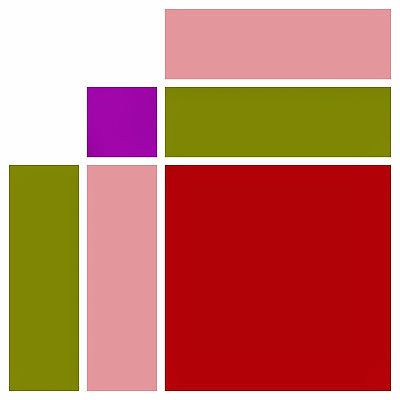
This image demonstrates the factoring of difference of squares:

x² - y² = (x + y)(x - y).

Let the larger square, made up of the red and purple square and the pink and gold rectangles, have a side length of x, so its area is x². And the small purple square have a side length of y, so its area is y².  Then the area in the remaining three pieces (red square and pink and gold rectangles) is x² - y².  Both rectangles have the same area, y × (x - y).  So all three of these regions have the same area:

• the horizontal rectangle made up of the gold and pink vertical rectangles and the red square
• the vertical rectangle made up of the gold and pink horizontal rectangles and the red square
• the original square, less the small purple square (area of x² - y²)

and that area is:

• (x - y)(x - y) + 2y(x - y), or
• (x - y + 2y)(x - y), or
• (x + y)(x - y)

So x² - y² = (x + y)(x - y).

Area of a Triangle

This image is a visual demonstration of the fact that the area of a triangle is one half of the base times its height.  Within the overall rectangle above, there are three main triangles of interest.  There's a blue one, made up of the two darker blue regions on the bottom plus the lighter blue region on the right side.  This right triangle has the same height as the overall rectangle and its base is the length of the overall rectangle.  Since the hypotenuse of the right triangle splits the rectangle into two equal areas, the area of the blue triangle is half the area of the rectangle, or A = 1/2 × base × height.

Alternatively, there's an acute triangle, made up of the two darker blue pieces plus the two darker yellow pieces on top of them.  This triangle also has a height that's the same as the overall triangle.  The altitude (white line from the bottom of the triangle to the top point) splits the overall rectangle into two smaller rectangles.  Each smaller rectangle has two smaller right triangles, each with one yellow piece and one blue piece, and both right triangles have areas that are half of that of their respective rectangles.  So, the area of the left small yellow & blue triangle (which is half of the area of its rectangle) + the area of the right small yellow & blue triangle (which is half of the area of its rectangle) = the area of the large yellow & blue triangle, which is half of the area of the overall rectangle.

Finally, there's the case of an obtuse triangle, played here by two darker yellow pieces plus the lighter yellow piece.  The big yellow triangle plus the green one together make up the other half of the overall rectangle (across the diagonal from the blue one).  By itself, the green triangle makes up half of the smaller left rectangle.  Therefore, the area of the yellow triangle has to be half of the smaller right rectangle, since the smaller left + smaller right rectangles make up the overall rectangle.  The area of the smaller right rectangle is its height (same as the height of the yellow triangle) × its width, which is the same as the base of the yellow triangle.  Once again, this shows that A = 1/2 × base × height.

Challenge Function

High school math teacher Mike Aben gave this challenge to his algebra class:

It turns out that f(x) is a rational function, that is, the ratio of two polynomials.  One way to see this is to realize that 1/(1/x) = x, so that by replacing “x” with “1/x” in the equation, a second equation would result.  The two can then be solved simultaneously, yielding an equation for f(x).

This got me to thinking about how I might adapt this idea into a fractal equation.  The x² in the challenge equation is similar to the z² + c in the Mandelbrot function, so I thought, let f(z) be such that 2f(z) – 3f(1/z) = z² + c, and iterate f(z) to get a fractal. After a few seconds, I realized that I could generalize this to:  let f(z) be such that Af(z) + Bf(1/z) = z² + c. As in Mike’s challenge, the function is a rational one. When iterated, it can yield a wide variety of structures and images, depending on the values of A, B, and n.

Here is my challenge:

And here is the function to be iterated:

Here are a few examples.  The first is a Mandelbrot set for 2f(z) - 4f(1/z) = z² + c.

The colored regions in the centers of the main cardioid and the surrounding disks are reflective of this being a rational function and represent areas where z approaches 0.

Here is a zoom into the center, for 9f(z) - f(1/z) = z³+ c.

And, in closing, this image and the one at the top of the page are Julias for the quadratic form of this function.

Pseudo-Bifurcation diagram of f(x) = ln(x*x)

Here's a pseudo-bifurcation diagram for f(x) = ln(x²).  It came up in a discussion on the math-fun mailing list about repeatedly hitting the "ln(x)" and then the "x²" buttons on a calculator.  The original observation was how the values jumped around instead of settling in to a fixed final value or cycle of values.  This image helps to explain why.  It's not a real bifurcation diagram because the values jump around too much to give a nice, coherent picture.  Instead, I've plotted the actual function values for each of 10 iterations. The plot is symmetrical about x = 0 and red line is at x ~ -0.7035, the location of the fixed point.  The blue lines are at x ~ -1.2985 and x ~ 0.5224, the values in the period-2 cycle.  The plot resembles a series of onion layers, giving an indication of the repelling orbits of this function.

 Romeo

Romeo and Juliett (and NATO and Fractals)

As everyone knows, Romeo and Juliett aren’t two star-crossed lovers, they are two of the code words in the NATO phonetic alphabet, or, more accurately, the International Radiotelephony Spelling Alphabet.  This is the spoken-word alphabet used by pilots, the military, and others who need to speak over radios and wish to minimize confusion due to similarly-sounding letters.  For example, instead of speaking the letters "m" or "n," the speaker would use the code words "mike" and "november," respectively.  The alphabet has a different-sounding word for each letter, from a-z:

Letter	Word	Letter	Word
a	alfa	n	november
b	bravo	o	oscar
c	charlie	p	papa
d	delta	q	quebec
e	echo	r	romeo
f	foxtrot	s	sierra
g	golf	t	tango
h	hotel	u	uniform
i	india	v	victor
j	juliett	w	whiskey
k	kilo	x	xray
l	lima	y	yankee
m	mike	z	zulu

Romeo and Juliett are the words for the letters r and j, respectively.

Imagine an admittedly silly radio conversation.  The sender wishes to communicate the letter "r."  She knows to use the phonetic alphabet and says, "romeo."  The receiver, not being too smart, asks for clarification.  So, the sender tries again.  After several botched communication attempts, the sender loses sight of her original desire and fixates on communicating "romeo."  So, she spells it:  "romeo, oscar, mike, echo, oscar."  Several more lacks of understanding, so she tries spelling the spelling words:  "romeo, oscar, mike, echo, oscar, oscar, sierra, charlie, alfa, romeo," etc.

At this point, we have all the fixin’s for a string-replacement sequence, so we’ll turn from radio communication to math.  A string replacement sequence is one built up in stages:  at each subsequent stage, characters from the previous are replaced with given strings.  Examples are the Thue-Morse sequence and the Fibonacci word.  In this case, we start with the letter r.  At each stage, every letter is replaced with its phonetic alphabet code word.  The first few stages are:

1. romeo
2. romeo oscar mike echo oscar
3. romeo oscar mike echo oscar oscar sierra charlie alfa romeo mike india kilo echo echo charlie hotel oscar oscar sierra charlie alfa romeo

(The spaces between words are just to improve readability and are not part of the sequence.)

A couple of things are apparent immediately.  First, the sequence of words grows pretty fast.  Each subsequent stage has about five times the number of letters as does the previous stage.  The 12th stage is almost 200 million letters long!

Second, the beginning of each subsequent stage is just the entirety of the previous stage.  This means that, when taken to the infinity stage, the resulting sequence of words is a self-referential fractal sequence.  It is self-referential in that it spells itself.  That is, if you were to spell each word, in order, using the phonetic alphabet, the result would be the same as reading the list.  This follows from how the sequence was created in the first place, by replacing each letter with its respective code word.  The fractal nature of the sequence means that the infinite sequence contains infinite copies of itself.  One way to see this is by reversing the creation process—replace each word with its first letter and you recover the sequence.  Alternatively, list the sequence in a column, each word below its predecessor.  Start with “romeo” and highlight it.  It has five letters, so count down five words and highlight “oscar” (it’s the third occurrence).   Count down five more words for the five letters in “oscar” to “mike” and highlight it.  Four more words (for the four letters in “mike”) to “echo,” and then four more words to another “oscar.”  The highlighted words are the original sequence.  In concept (with an infinite sequence), you could delete the non-highlighted words and repeat this process forever, always coming back to the same sequence.

• romeo
• oscar
• mike
• echo
• oscar
• oscar
• sierra
• charlie
• alfa
• romeo
• mike
• india
• kilo
• echo
• echo
• charlie
• hotel
• oscar
• oscar
• sierra
• charlie
• alfa
• romeo
• …

So what about juliett?  Juliett has a similar sequence, beginning:  juliett uniform lima india echo tango tango uniform november india foxtrot oscar romeo mike lima india mike alfa india november delta india alfa echo charlie hotel oscar tango alfa november golf oscar tango alfa november golf oscar.  It too grows quickly, quintupling the number of letters at each stage.  By its 12th stage, this sequence has over 350 million letters.  Interestingly, the letter “j” only occurs once in this infinite sequence, at the very beginning.  That’s because there are no code words in the alphabet that contain j, aside from juliett, which begins with j.  The self-reference and fractal stuff about the romeo sequence hold for juliett’s, as well.

And what does all this have to do with the image at the top of this post?  For either sequence (or for any of the other 24), each letter can be replaced with a number from 1 (for "a") to 26 (for "z").  These numbers can then be used to create images.  To see how, look at the picture below.  Imagine that you’re at the “start” point and getting ready to draw a line off to the right.  Instead, you turn left 45 degrees and draw a line one unit long.  Then, turn left again by 45 degrees and draw another line.  Repeat this six more times and you’ll have the red octagon.

Increase the turn angle to 60 degrees and you’ll get the hexagon.  The other shapes come from turning left 72, 90, and 120 degrees, respectively, before drawing the line.  And the star at the bottom comes from turning right 144 degrees before drawing.  The point is that, this process of turning a set amount and then drawing a line can lead to many different images.

For “Romeo,” at the top of this page, the turn was about 179 degrees left (almost straight back on itself) for each of 100,000 steps.  However, the lengths of the lines varied.  Each segment was from 1 to 26 units long, depending on the corresponding letter in the romeo sequence.  That is, the first segment was 18 units long, as r is the 18th letter.  Below is “Juliett.”

Here, each segment is the same length, but the amount of turning varies.  Each turn is about 179 degrees multiplied by the number for the letter in the juliett sequence.

These last two images, “Romeo and Juliett I” and “Romeo and Juliett II,” use both sequences in determining the amount to turn and the lengths of the segments.

Romeo and Juliett I

 

Romeo and Juliett II

    

Thirteen

Four years ago, I wrote a blog post (What to do with 1 million iterations?) about zooms into the Mandelbrot set that require a lot of iterations (1 million, in that case), but that weren’t deep zooms.  I also featured the Color of the Year for 2009, mimosa.  Now, in honor of 2013, I return with a different zoom, featuring 2013’s Color of the Year, emerald.

This image, “Thirteen,” pays homage to its namesake number through a progression of disks with 13-armed spirals.

Each disk in the Mandelbrot set has associated with it, a fraction in lowest terms.  Around the main cardioid, the numbering starts with 0/1 at the cusp, around the top (1/3 represents the largest disk on top), to the left edge (disk 1/2), around the bottom (2/3 for the largest on the bottom), and finishing up with 1/1 back at the cusp.  The largest disk between any two disks has a fraction that is between the two disks' fractions, in a special way.  If the two surrounding disks have fractions a/b and c/d, then the largest between them has the fraction (a+c)/(b+d).  For example, between both extremes of 0/1 and 1/1, lies the largest disk, 1/2, or (0+1)/(1+1).  Between 1/2 and 0/1 lies the 1/3 disk on top, and so on.  Working clockwise down to the cusp, the largest disks are 1/4, 1/5, 1/6, etc.  Way down there is 1/13:

Its “headdress,” or the system of arms emanating from the top of the disk, reflects the fraction 1/13, in that there are 13 arms.  Label the one coming out of the disk as arm 0 and count clockwise.  The first arm, arm 1, is the most prominent of the bunch.  Also, the lengths of the arms vary smoothly from one to the next.  This will be important later.

Back up the cardioid is the 2/13 disk.  It is the largest disk between those for 1/6 and 1/7.

This disk also has 13 arms in its headdress.  Again, counting clockwise from 0 (the arm coming out of the disk), arm 2 is the most prominent.  This time, instead of the arms lengths varying smoothly, they oscillate, with the even-numbered arms being longer than the odd-numbered arms.

Moving back up the cardioid to the 1/3 disk, we encounter the 3/13 disk.

This one is a bit trickier to find:  first, find the 2/9 disk, between 1/4 and 1/5.  Then, between the 2/9 and 1/3 disks is the 3/13 disk.  It also has 13 arms and the third one is the most prominent.  Notice here how the arms get longer in groups of three.

It seems then, that every disk with a fraction of p/q has q arms emanating from its headdress, the pth arm is the most prominent, and arms whose numbers are multiples of p are longer than their neighbors.

Each disk has disks of its own, and they have disks, and so on, down to infinity.  These sub-disks carry with them their heritage of the disks that came before them.

Here is the 2/13 disk of the 1/13 disk (for sub-disks, 0/1 and 1/1 are at the base where it connects to its parent disk).  Immediately above the disk, and darker in this image, are the arms reminiscent of the 2/13 disk, 13 in number with arm 2 being the most prominent.  Following this arm outward leads to the spiral remnants of the 1/13 disk.  Since this disk is a child of the 1/13 disk, as are all in this image, all have the same 1/13 spiral structure at the ends of their arms.  However, their inner structure depends on their own fractions.

This final example shows how the structure in “Thirteen” came to be.  The largest disk at the bottom-right of this image is the 3/13 disk of the 2/13 disk of the 1/13 disk of the main cardioid.  The 3/13 structure is clear in gray immediately above the disk.  Arm 3 extends toward the top of the image, bearing a bright white spiral center of the 2/13 arms.  Arm 2 of this spiral reaches almost to the top of the image.  Very small is the 1/13 spiral, culminating in the tip of arm 1, just barely visible.

As the chain of disks gets longer, the structures become increasingly compressed and tightly wound, in order to incorporate the lengthening train of parental arms.  Ultimately, the image becomes filled with spiral structure.  This reflects the fact that the boundary of the Mandelbrot set has a fractal dimension of 2 and is an area-filling curve.

19 61

If you’ve played with fractions and decimals (and who hasn’t?), then you probably know that 7 is a special number.  The reciprocal of 7, 1/7, has a decimal expansion that repeats.  That’s not special—most fractions do.  However, what makes 7 (or 1/7) more special is that the block of repeating digits is as long as is possible (one less than the denominator--6 digits, in this case).  Also, the fractions 2/7 through 6/7 have decimal expansions that repeat with the same block (bolded below):

• 1/7 = 0.142857142857142857142857142857…
• 2/7 = 0.285714285714285714285714285714…
• 3/7 = 0.428571428571428571428571428571…
• 4/7 = 0.571428571428571428571428571428…
• 5/7 = 0.714285714285714285714285714285…
• 6/7 = 0.857142857142857142857142857142…

Alternatively, we can look at the repeating blocks as different, but as cyclic permutations of the block for 1/7.  That is, the block for 1/7 is 142857.  For 2/7, it is 285714, which is just 142857, shifted by two spots.  For 3/7, 428571 is shifted one spot from the original.  Likewise for the other three fractions.  This makes 7 a cyclic prime.  It’s not the only one; there are lots.  For a list, see entry A001913 in the Online Encyclopedia of Integer Sequences.

It turns out that 19 and 61 are also cyclic primes.  Just as 7 has six numbers in its repeating block, 19 has 18 and 61 has 60.  The blocks for 1/19 and 1/61 are:

·         1/19 = 052631578947368421…

·         1/61 = 016393442622950819672131147540983606557377049180327868852459…

Since I was born in 1961, I thought I’d try to do something with that.  It seemed reasonable to try to fit all of the fractions into an 18 x 60 box, those with a denominator of 19 being columns 18 rows long, and those with a denominator of 61 being rows 60 columns long.  For example, the blocks for fractions m/7 can fit into a 6 x 6 square; here are four of them:

		3/7		6/7
		4		8
		2		5
2/7	2	8	5	7	1	4
		5		1
4/7	5	7	1	4	2	8
		1		2

Alas, for 19 and 61, it’s not quite that simple.  There are only 18 different decimal expansions for fractions of the form m/19, not 60, and there are 60 decimal expansions for fractions of the form m/61, not just 18.  Also, the actual numbers don’t generally line up, like they do for m/7.  But, I was able to find one case in which 21 blocks of repeating decimals fit, and another in which 24 blocks fit.  Here’s the upper left corner of the 21-block box:

							14/19	11/19		2/19
							7	5		1
37/61	6	0	6	5	5	7	3	7	7	0
49/61	8	0	3	2	7	8	6	8	8	5
							8	9		2
1/61	0	1	6	3	9	3	4	4	2	6

This shows that the decimal expansion of 14/19 begins 0.73684, and that of 37/61 begins 0.6065573770.  Note that both share the 3 that is in the second row, seventh column.  One trick in setting up this box was ensuring that, whenever a row fraction and a column fraction share the same cell, that numeral is correct in both expansions.

Another challenge was how to present this an in aesthetically interesting fashion.  I came up with a solution, but will leave it to you to decide how interesting it is.  Rather than just writing the numerals, I used modified rose curves to represent them.  In the 21-block case, they are all shown using this alphabet, which shows 0, 1, 2, 4, and 8:

In the 24-block case, I tweaked the design a bit.  Also, I decided to render those numbers in the intersection cells (like 3, above, which is shared by 14/19 and 37/61) in negative.  Here are the symbols for 3, 5, 6, 7, and 9:

Now that you know what the symbols mean, you can read the image and there’s no need for labels, right?  So, without further ado, I present “19 61 a” and “19 61 b.”

19 61 a

19 61 b

Space-Filling Curves from Polygonal Dissections

When I was a kid, I would spend hours drawing on graph paper, breaking down rectangles into smaller rectangles and triangles, and triangles into smaller triangles and rectangles.  Many years later, I learned about fractal tessellations (the result of such decompositions after an infinity of cycles) and wrote formulas to do that, leading to images like this.

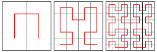
Recently, I returned to these dissections as methods for generating space-filling curves.  For example, the Hilbert curve can be created by dissecting a square into four smaller squares, and connecting the centers:

In the first panel, the original square (thick black line) is dissected into four squares (thin black lines), whose centers are connected with the red curve.  This process is repeated, wherein every square from the previous iteration is dissected into four smaller squares.  The centers of all these new squares are connected with a line that is four copies of the previous curve, shrunken and rotated, and the result is a space-filling fractal curve.

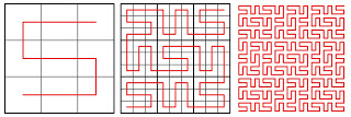
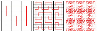
While the Hilbert curve is based on a 2 × 2 grid of four squares, other grids can be used.  Here are the first three iterations of two curves based on 3 × 3 dissections of the square (in the third iteration, the squares have been left off for clarity):

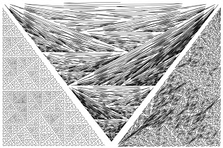
The concept is quite general and can be extended to other shapes:  develop a scheme for dissecting a base shape into smaller shapes and draw a curve connecting the centers.  For practical reasons, I’ve kept my investigations to triangles and convex quadrilaterals (not necessarily rectangles).  And for aesthetic reasons, I’ve decided that my curves will not cross themselves (the so-called “self-avoiding” curve).  Here are three cases of dissecting a triangle into three smaller triangles.  Note the appearance of shading, especially in the middle case.

Some very interesting opportunities arise when two different shapes are combined.  For example, a quadrilateral can be broken up into triangles and quadrilaterals, each of which can be further decomposed into more triangles and quadrilaterals.

This technique has proven very fruitful for me and I’ll soon have more examples up on my website.